Inverse Kinematics and Jacobian for Serial Manipulators

Elissa Ledoux

4 Inverse Kinematics and Jacobian for Serial Manipulators

Elissa Ledoux

1) Inverse Kinematics

Theory

Inverse kinematics (IK) is the mathematical mapping from end effector pose (x, y, z, roll, pitch, yaw) to joint positions (d’s, $\theta$ ‘s).

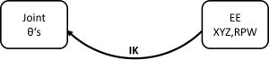
Similarly to forward kinematics, this relationship is independent of force and torque and assumes that each joint in the chain has one degree of freedom (or is two joints). IK is more difficult than FK for serial robots because multiple solutions are possible, but it is easier than FK for parallel robots because only one solution is possible.

The goal of IK is to find all solutions to the base-to-tip transformation $T_n^0 (\theta_1,\theta_2,...\theta_n) = \begin{bmatrix} R_n^0 & o_n^0 \\ 0 & 1 \end{bmatrix}$ . The method is to take the first three rows of $T_n^0$ and solve for all d’s and $\theta's$ . This results in 12 equations (one per element of the reduced 3×4 matrix) and n unknowns. Typically n < 6 so a solution is almost always possible. Closed-form analytical solutions (as opposed to numerical solutions) are ideal. The possible cases for a serial manipulator are:

no solution (point is outside robot’s workspace)
one solution (point is on edge of workspace)
multiple solutions (point is inside workspace)
impossible solutions (point is inside workspace but not possible for the end effector to reach at the given orientation, such as points inside the robot itself or that would require to the robot to do contortions)

For a detailed explanation of inverse kinematics, watch the video below. A downloadable slide deck corresponding to the videos but not annotated is available here: IK Basics Slides

Video: Inverse Kinematics Intro (click link for closed-caption version)

This theory is applied in examples below showing how to determine the inverse kinematics for two robots, one in 3D space (an RRP Stanford Manipulator), and one in 2D space (an RR planar manipulator).

Quick Quiz

Examples

The video below demonstrates how to solve the inverse kinematics for an RRP Stanford Manipulator.

Video: IK Example – RRP Stanford Manipulator (click link for closed-caption version)

The video below demonstrates how to solve the inverse kinematics for a 2-link RR manipulator.

Video: IK Example – Two Link (RR) Manipulator (click link for closed-caption version)

2) Jacobian

Theory

The Jacobian is a matrix expressing the derivative of end effector position with respect to joint variables:

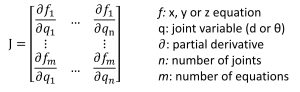
Each element is the derivative of the pose variable with respect to the joint variable corresponding to each row and column.

In 3D space, the Jacobian is a 6×6 matrix. The rows represent the end effector pose variables: x, y, z, roll, pitch, yaw from top to bottom. The columns represent the joint variables: $\theta$ or d for each joint.
In 2D space, the Jacobian is a 3×3 matrix (or occasionally a 2×2 if there are only 2 joints). The rows represent the end effector pose variables: x, y, and yaw from top to bottom. The columns represent the joint variables: $\theta$ or d for each joint.

For forward and inverse kinematics (position), the Jacobian relates tip pose to joint positions:

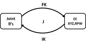
For derivative kinematics (velocity), the Jacobian relates task space velocities (end effector) to joint space velocities (joints):

$J \dot q = \xi$ or $J \dot\theta = \dot X$

Figure 4.4: Jacobian and Velocity Relationships

For a detailed explanation about the Jacobian, watch the video below. A downloadable slide deck corresponding to the video above but not annotated is available here: Jacobian Theory Slides Feel free to print and take notes as you follow along.

Video: Jacobian Introduction (click link for closed-caption version)

For an n-link robot with joint variables $q_1$ … $q_n$ , and a forward kinematics homogeneous transformation matrix $T_n^0$ , there are two methods for finding the Jacobian:

Basic method (for simple robots, n < 3)
Formula method (for complex robots, n > 3)

The next sections will walk through the steps to find a Jacobian for a two-link RR robot using first the basic method and then the formula method.

Basic Method and Example

For an n-link robot with joint variables $q_1$ … $q_n$ , and a forward kinematics base-to-tip homogeneous transformation matrix $T_n^0 = \begin{bmatrix} R_n^0 & o_n^0 \\ 0 & 1 \end{bmatrix}$ , the procedure to solve using the basic method is:

Write position equations for the tip in the world frame (base frame) $o_n^0$
Take the derivative to find velocity
Put the equations in matrix form $\dot X = J \dot \theta$

The video below demonstrates how to derive the Jacobian for a 2-link RR manipulator using the basic method. A downloadable slide deck corresponding to the video example but not annotated is available here: RR-Robot-Jacobian-Basic-Method-Slides Feel free to print and take notes as you follow along.

Video: Two Link RR Manipulator Jacobian Example – Basic Method (click link for closed-caption version)

Formula Method and Example

For an n-link robot with joint variables $q_1$ … $q_n$ , and a forward kinematics base-to-tip homogeneous transformation matrix $T_n^0 = \begin{bmatrix} R_n^0 & o_n^0 \\ 0 & 1 \end{bmatrix}$ , the procedure to solve using the formula method is:

0. Determine the forward kinematics matrix (if not given).
1. Write position equations for all joint origins in the world frame $o_i^0$
2. Write all joint axis vectors $z_i$
3. Do math by category ( $J_v$ , $J_\omega$ , revolute joints, prismatic joints) as follows:

For the linear Jacobian $J_v$ : assume all joints are fixed and look at the end effector velocity:

$J_v = \begin{cases} z_{i-1} \times (o_n - o_{i-1}): revolute \\ z_{i-1} : prismatic \end{cases}$

For the angular Jacobian $J_\omega$ : look at the rotation of frame i relative to frame i-1 :

$J_\omega = \begin{cases} z_{i-1} : revolute \\ 0 \: (3 \times 1 \: matrix) : prismatic \end{cases}$

The video below demonstrates how to derive the Jacobian for a 2-link RR manipulator using the formula method. A downloadable slide deck corresponding to the video examples but not annotated is available here: RR Robot Jacobian Formula Method Slides Feel free to print and take notes as you follow along.

Video: Two Link RR Manipulator – Formula Method (click link for closed-caption version)

The video below demonstrates how to derive the Jacobian for an RRP SCARA robot using the formula method.

Video: RRP Robot Jacobian Example (click link for closed-caption version)

Quick Quiz

Applications

The Jacobian has many applications in robotics. It can be used to:

Find singular configurations of a robot
Plan and execute motion trajectories
Coordinate motion (position, velocity, and acceleration)
Derive dynamic equations of motion
Find required joint torque given end effector forces and torques
Resolve redundancies (when there are more joints than DoF of the operating space)

The Jacobian can be used with inverse kinematics to determine the required joint speeds to drive a robot’s tip at a certain speed. For example, if you are programming a welding robot, and the robot must weld along a line at a constant tip velocity, the joint speeds will not necessarily be constant. However, using the equation $\dot q = J^{-1}* \dot X$ , you can calculate the required joint speeds for the entire path.

The Jacobian can be used with forward kinematics to determine velocity at any point on the robot’s arm. In this situation, you would place a point p at the desired location on the arm to track, and write the Jacobian up to that point using the formula method with p instead of $o_n$ . Then using the equation $\dot X = J \dot q$ , with the new Jacobian, you can determine velocity of the point in question.

The Jacobian can be used to relate joint torques and end effector forces using the equation $\tau = J^T F$ , where $\tau$ represents joint torques (n x 1 vector), J is the Jacobian (6xn), and F is the end effector “wrench” (6×1 vector of xyz forces and roll-pitch-yaw torques). The exponent T means “transpose”: switching the rows and columns of a matrix. So to apply a certain force at the end effector, the joint torque can be easily calculated using that formula. To determine force applied for known joint torque, perform the inverse: $F = (J^T)^{-1} * \tau$ . The Jacobian in this instance does not need to be square like it does for kinematics.

3) Singularities

Theory

Manipulator singularities occur when joint axes align or lock. This is a bad situation! Singularities result in the manipulator losing a degree of freedom and therefore the ability to move in a certain direction at that instant. Bounded end effector velocities result in infinite joint velocities, and bounded joint torques result in unbounded end effector force and torque. Finally, there are infinite possible solutions to the inverse kinematics for that end effector pose. Singularities should be avoided at all costs, otherwise the robot could break.

For a detailed explanation of robot singularities, watch the video below.

Video: Robot Singularities (click link for closed-caption version)

In 2D space, singularities occur when the robot’s joint axes lock out, yielding only one solution to the robot’s IK. These are points on the edge of the workspace (when the robot is stretched out at full extension), or when two of the links are doubled back on each other, completely aligning.

In 3D space, singularities occur when joint axes align and there are infinite solutions for the robot’s IK. For a standard 6-axis robot, this can occur when joints 1, 4, and 6 (or some combination of those) align. For a visualization of a standard 6R robot moving to near-singularity poses, watch the video below from Mecademic.

Video: What are robot singularities? by Mecademic

Mathematically, singularities occur when the determinant of the Jacobian = 0. So if J = 0, and desired tip speed is a number represented by $\dot X$ , you can see that joint speeds $\dot q$ would try to shoot to infinity to achieve that in the equation $\dot X = J \dot q$ .

There are two methods to find singularities:

Inspection
Calculation

These methods are explained below and illustrated with examples. A downloadable slide deck corresponding to these video examples but not annotated is available here: Singularity Examples Slides Feel free to print and take notes as you follow along.

Examples

To solve singularities by calculation,

Write the FK position equations for the robot tip
Take the derivative to find velocity
Put the velocity equations in matrix form $\dot X = J \dot q$
Set det(J) = 0 and solve for joint variables q

The video below demonstrates how to find the singularities for a 2-link RR manipulator using math.

Video: 2-Link RR Manipulator Singularity Example (click link for closed-caption version)

To solve singularities by observation:

Look at the robot’s joint alignment
Visually determine the singularity angles

The video below demonstrates how to find the singularities for two different PR robots by observation and prove them with math.

Video: PR Robot Singularities (click link for closed-caption version)

Quick Quiz

4) MATLAB Programming

In order to program a robot to follow a path, knowledge of both the forward and inverse kinematics is necessary. Depending on the degrees of freedom of the robot and dimensions of the operating space (e.g. 2D or 3D), one may be able to control either just position or both position and orientation. A standard 6-axis robot has 6 DoF and operates in 3D space; therefore it is possible to control the entire pose: x/y/z position and roll/pitch/yaw orientation. (Note that this does not mean all poses are possible; the robot must always operate within its workspace.) For a simpler Cartesian 3P robot (like a 3D printer), it is possible to control x/y/z position, but not orientation, because such a robot cannot rotate its end effector. A 2R planar robot can control x/y position only, due to having only 2 DoF, but a 3R planar robot can control both x/y position and yaw orientation (angle around z) because it has 3 DoF. For most robots, the number of degrees of freedom corresponds to the number of controllable pose variables.

As seen above, the inverse kinematics can be solved either algebraically or numerically in order to simulate the robot’s motion. If an algebraic solution is possible, this is the more accurate method. If the solution cannot be found algebraically, the Jacobian can be used to solve the joint positions numerically. This is computationally longer and less accurate, but it is a much easier method for solving complicated robots if done in silico (computer program) rather than by hand. The subsections below show how to solve inverse kinematics for a PR robot both algebraically and by hand, and how simulate the robot in MATLAB both ways.

Algebraic Solutions

An algebraic solution is one in which unknown variables can be solved for manually, and expressions for each unknown variable can be found independent of the others. This method is typically used for simple robots with three or fewer DoF. Examples of algebraic solutions for inverse kinematics are shown above in Part 1 of this chapter.

For this example, we will consider a simple PR robot: one prismatic joint and one revolute joint, the first one in PR Robot Singularities video above.

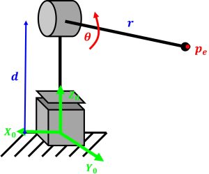
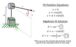
Planar PR robot — Figure 4.5: PR Planar Robot

This robot operates in the YZ plane, where Z points up and Y points to the right. We can write the forward kinematics as follows:

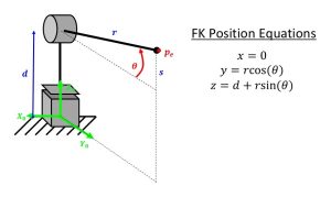
PR Forward Kinematics Equations — Figure 4.6: PR Robot Forward Kinematics Equations

Then we can rearrange these equations to solve for the inverse kinematics algebraically:

PR algebraic solution IK — Figure 4.7: Algebraic Inverse Kinematics Solution for PR Robot

In order to simulate the robot with a computer program, the following steps are required, and can be used as an outline for the code:

Define knowns, constants, and desired end effector path (x/y/z/roll/pitch/yaw, whatever is applicable)
Preallocate arrays to store calculated values for the IK
Begin a for loop to start calculations for each frame
- Calculate the joint values (IK) using the algebraic equations derived
- Calculate the joint and tip locations in space using FK equations
- Define arrays of points to plot (matrices of x, y, and z points)
- Plot the robot
End the for loop

An example code using the algebraic method to simulate the PR robot is shown below. This book software cannot read or attach .m files, so a downloadable version is not possible, but you may copy and paste from the textbox.

Example Algebraic Code for PR Robot Simulation

%% PR manipulator simulation (Algebraic solution)
% PR robot tracing path
% Robot operates in YZ plane
% Elissa Ledoux ENGR 4501 Spring 2025

clc
clear
close all

% define constants (arbitrary if not given)
r = 0.5; % link lengths (m)
nsteps = 50; % number of steps

% define desired path for end effector (m)
ystart = 0.5;
ystop = -0.48;
pdesy = linspace(ystart,ystop,nsteps);
pdesz = .7 - (pdesy-0.1).^2; % path option 1 % pdesz = 0.5 + 0.2*sin(pdesy*10*pi); % path option 2
pdes = [pdesy;pdesz]; % waypoints (m)

% preallocate arrays
tip = zeros(2,nsteps); % actual tip path (y and z)
d = zeros(nsteps,1); % prismatic joint
th = zeros(nsteps,1); % revolute joint

% calculate kinematics
for i = 1:nsteps

% solve algebraically
th(i) = acos(pdesy(i)/r);
d(i) = pdesz(i) - r*sin(th(i));

% check solution
y = r*cos(th(i));
z = d(i) + r*sin(th(i));

% calculate points to plot (location of each joint)
tip(:,i) = [y;z];
j1y = 0; j1z = 0; % joint 1
j2y = 0; j2z = d(i); % joint 2
jey = r*cos(th(i)); jez = d(i)+r*sin(th(i)); % end effector
Y = [j1y, j2y, jey];
Z = [j1z, j2z, jez];

% plot robot
figure(1)
clf
hold on
plot([j1y,j2y],[j1z,j2z],'k','LineWidth',3)
plot([j2y,jey],[j2z,jez],'r','LineWidth',3)
plot(j1y,j1z,'ksq','MarkerSize',10,'MarkerFaceColor','k')
plot(j2y,j2z,'ro','MarkerSize',10,'MarkerFaceColor','r')
plot(jey,jez,'b*','MarkerSize',10)
plot(tip(1,1:i),tip(2,1:i),'b')
xlim([-1 1]); xlabel('Y (m)')
ylim([-.5 1.5]); ylabel('Z (m)')
axis square
title('PR Planar Manipulator')

end

Numerical Solutions

A numerical solution is one in which unknown variables cannot be solved for manually, and rather are done using the guess-and-check method known as “Newton’s method” or the “Newton-Rhapson method.” This method is typically used for complicated robots with three or more DoF. A numerical solution is done using the robot’s Jacobian to iteratively guide guesses for the joint values to until they converge, resulting in a solution for the IK. IF YOU ARE NEW TO NEWTON’S METHOD, STUDY SECTION 5 BELOW BEFORE PROCEEDING SO YOU WILL NOT BE UTTERLY LOST.

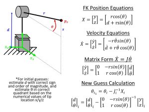
For this example, we will consider a the same RP robot as before, with the same forward kinematics, and solve for the inverse kinematics numerically using a while loop (guess-and-check while error is greater than a tolerance value and the solution for joint positions converges). This requires deriving the Jacobian of the robot by hand and choosing an initial guess for the joint values before using a computer program to solve the system numerically. The velocity, Jacobian, and guess iteration formulas for this PR robot are shown in the figure below:

PR robot velocity and Jacobian — Figure 4.8: Jacobian and Velocity Kinematics Equations of the PR Robot

In order to simulate the robot with a computer program, the following process is required (similarly to the algebraic solution but with additional steps), and can be used as an outline for the code:

Define knowns, constants, and desired end effector path (x/y/z/roll/pitch/yaw, whatever is applicable)
Preallocate arrays to store calculated values for the IK
Choose initial guesses for the joint values (these must be reasonably accurate or the program will get stuck in an infinite loop and never solve. I.e. ensure $\theta$ is in the correct quadrant and $d$ is on the correct order of magnitude)
Begin a for loop to start calculations for each frame
- Find the current tip position F using FK based on the initial guesses
- Calculate the magnitude of position error
- Start a while loop to iterate guesses
  - Calculate the Jacobian using the current guesses
  - Calculate new joint values using $\theta_{new} = \theta{old} - J^{-1}F$
  - Find the new tip position using FK based on the new guesses
  - Calculate the magnitude of position error
- Exit the while loop once guesses are close enough (error within tolerance)
- Calculate the joint and tip locations in space using FK equations with the correct guesses
- Define arrays of points to plot (matrices of x, y, and z points)
- Plot the robot
End the for loop

An example code using the numerical method to simulate the PR robot is shown below. This book software cannot read or attach .m files, so a downloadable version is not possible, but you may copy and paste from the textbox.

Example Numerical Code for PR Robot Simulation

%% PR manipulator simulation (Numerical Solution)
% PR robot tracing path
% Robot operates in YZ plane
% Elissa Ledoux ENGR 4501 Spring 2025

clc
clear
close all

% define constants (arbitrary if not given)
r = 0.5; % link lengths (m)
nsteps = 50; % number of steps
dt = 0.1; % timestep
vee = 1; % end effector velocity (m/s)
tol = 10^(-3); % accuracy tolerance (m)

% define desired path for end effector (m)
ystart = 0.5;
ystop = -0.48;
pdesy = linspace(ystart,ystop,nsteps);
pdesz = .7 - (pdesy-0.1).^2; % path option 1
% pdesz = 0.5 + 0.2*sin(pdesy*10*pi); % path option 2
pdes = [pdesy;pdesz]; % waypoints (m)

% preallocate arrays
tip = zeros(2,nsteps); % actual tip path (y and z)
d = zeros(nsteps,1); % prismatic joint
th = zeros(nsteps,1); % revolute joint

% initial guesses (joint positions)
d_guess = 0.2; d(1) = d_guess;
th_guess = pi/10; th(1) = th_guess;

% calculate kinematics
for i = 1:nsteps
c = 0; % counter

% find current point using FK (use basic, DH, or product of exp method)
y = r*cos(th(i));
z = d(i) + r*sin(th(i));
pcur = [y;z];

% find error
errvec = pdes(:,i)-pcur;
err = norm(errvec);

% solve numerically (guess-and-check Newton's method)
while err > tol

% find Jacobian (2D) (use basic or formula method)
J = [0, -r*sin(th_guess); ...
1, r*cos(th_guess)];

% find velocities of end effector and joints
xdot = vee*errvec;
qdot = J\xdot;

% calculate new joint positions
q = [d_guess; th_guess]+qdot*dt;
d_guess = q(1); th_guess = q(2);

% find current point using FK (use basic, DH, or product of exp)
y = r*cos(th_guess);
z = d_guess + r*sin(th_guess);
pcur = [y;z];

% find error
errvec = pdes(:,i)-pcur;
err = norm(errvec);

% update counter
c = c+1;
end

% save correct joint positions
d(i) = d_guess;
th(i) = th_guess;

% calculate points to plot (location of each joint)
tip(:,i) = [y;z];
j1y = 0; j1z = 0; % joint 1
j2y = 0; j2z = d(i); % joint 2
jey = r*cos(th(i)); jez = d(i)+r*sin(th(i)); % end effector
Y = [j1y, j2y, jey];
Z = [j1z, j2z, jez];

% plot robot
figure(1)
clf
hold on
plot([j1y,j2y],[j1z,j2z],'k','LineWidth',3)
plot([j2y,jey],[j2z,jez],'r','LineWidth',3)
plot(j1y,j1z,'ksq','MarkerSize',10,'MarkerFaceColor','k')
plot(j2y,j2z,'ro','MarkerSize',10,'MarkerFaceColor','r')
plot(jey,jez,'b*','MarkerSize',10)
plot(tip(1,1:i),tip(2,1:i),'b')
xlim([-1 1]); xlabel('Y (m)')
ylim([-.5 1.5]); ylabel('Z (m)')
axis square
title('PR Planar Manipulator')

end

A more detailed and downloadable outline for code logic including pose control (position and orientation both) is available here: Pose Control Logic

5) Review of Newton’s Method for Numerical Solutions

Newton’s method, or the Newton-Rhapson method, is a way to solve equations numerically, by finding roots or unknowns of a function or system of equations using a guess-and-check procedure. In advanced kinematics courses, it is used to solve and simulate mechanisms such as closed-chain or hybrid-chain linkages using vector loop equations. In robotics, Newton’s method can also be used to simulate both parallel and serial robots using forward and inverse kinematics.

The basic process is:

Make an initial guessG of values for the unknown variables
Calculate the value of the function F using the guess G
Check if the function value F nears zero. If so, stop. The guess is correct. If not, continue to step 4.
Calculate the derivative (Jacobian) J of the function and plug in the guess values.
Calculate a new guess G using the formula $G = G - J^{-1}F$
Repeat steps 2-5 until solved

An explanation of the theory as well as a simple example using a scalar equation and single unknown variable is in this video: Newton’s Method Explained + Example.

The process above can be followed to solve the equation using a computer program rather than by hand. A video tutorial on how to do this is here: Programming Newton’s Method in MATLAB.

If more than one variable must be solved for, such as multiple unknown joint values of a robot, matrices must be used instead of scalars. An explanation of how to set up matrices for a system of two equations and two unknowns for a parallel closed-chain mechanism is in this video: Four Bar Linkage Solution Newton’s Method.

This completes the review, and you are now ready to return to Part 4 of this chapter to solve and simulate a robot in Matlab numerically.

License

Icon for the Creative Commons Attribution-NonCommercial-ShareAlike 4.0 International License

Robotics and Controls Engineering Copyright © by Hongbo Zhang; Elissa Ledoux; and Vishwas Bedekar is licensed under a Creative Commons Attribution-NonCommercial-ShareAlike 4.0 International License, except where otherwise noted.

1) Inverse Kinematics

Theory

Quick Quiz

Examples

2) Jacobian

Theory

Basic Method and Example

Formula Method and Example

Quick Quiz

Applications

3) Singularities

Theory

Examples

Quick Quiz

4) MATLAB Programming

Algebraic Solutions

Numerical Solutions

5) Review of Newton’s Method for Numerical Solutions

License

Share This Book