Model Predictive Controller

Hongbo Zhang

14 Model Predictive Controller

Hongbo Zhang

1) Overview of Model Predictive Control

A Model Predicative Controller (MPC) is an optimal controller. This controller is used in practical control applications to not only control a system but also thoroughly consider the constraints of the system. MPC has been extensively used for process industries, power systems, automotive, and aerospace engineering. Interestingly, MPC also accommodates filtering the noise in a system to ensure noises would not adversely impact the system control performance.

$\newline$

A discrete state-space model for MPC is typically represented as:

$x(k+1) &= Ax(k) + Bu(k) + B_d d(k) + w(k)$

$y(k) &= Cx(k) + v(k)$

where:

x(k) is the state vector at time step k .
u(k) is the control input vector.
d(k) is the disturbance vector.
y(k) is the output vector.
A, B, Bd, and C are matrices that define the system dynamics.
w(k) and v(k) are process and measurement noise, respectively.

Figure 14.1 shows an example of random noises of a system.

Figure 14.1: A control system with random noises.

Such a discrete state space model is similar to the state space modeled previously. A notable difference, however, does exist. In contrast to the previous method, where the noises of the system are not explicitly considered, with this model, the noises of the system (including w(k), the process noise, and v(k), the measurement noise), are well considered.

$\newline$

Of these two different types of noises considered, the process noises w(k) are the noises embedded in the system. These can be illustrated through an example. Given an autonomous driving system, the system noise refers to the road surface variation, wind gusts, sensor inaccuracies, and actuator imperfections. On the other hand, an example of the measurement noises v(k) include the random errors or disturbances that affect the accuracy of measurements taken by sensors or instruments. More specifically, the measurements noises include thermal measurement noise, quantization noise (for the digital systems when continuous signals are converted to the discrete digital values.), the shot noise (noises associated with electric charge), environmental noise (such as electromagnetic interference), interference from other signals (such as radio frequency interference (RFI) and electromagnetic interference (EMI)), and human error.

2) Using a Kalman Filter to Reduce Noise

In order for MPC to perform optimal control, the noise of the system needs to be removed. MPC achieves noise filtering through the use of a Kalman filter or extended state observer (ESO). In our book, we will focus on the use of a Kalman filter to estimate the states and disturbances. To use a Kalman filter to extract noise from the system, the following the steps are needed.

$\newline$

The MPC is an optimal controller. Therefore, it involves a few steps to solve the optimization problem.

(A) Prediction Step:

Predict the next state:

$\hat{x}(k+1|k) = A \hat{x}(k|k) + B u(k)$

Predict the error covariance:

$P(k+1|k) = A P(k|k) A^T + Q$

Here, P is the error covariance matrix and Q is the process noise covariance.

(B) Update Step:

Compute the Kalman gain:

$K(k) = P(k|k-1) C^T (C P(k|k-1) C^T + R)^{-1}$

Update the state estimate:

$\hat{x}(k|k) = \hat{x}(k|k-1) + K(k) (y(k) - C \hat{x}(k|k-1))$

Update the error covariance matrix:

$P(k|k) = (I - K(k) C) P(k|k-1)$

Here, R is the measurement noise covariance.

$\newline$

The key idea of the Kalman filter is to compute the Kalman gain K and update the state estimate by the introduction of the error of covariance. Following the precise estimate of the state, it becomes possible to reject the noises from the system.

Figure 14.2: The control system with random noises removed. The orange curve shown in the figure represents the filtered noises from the system.

3) Model Predictive Control (MPC) Modeling

In this section, let us explore MPC modeling without noise. Following the use of the Kalman filter to filter out the noise from the system and estimate the true states, the MPC solver starts to solve the quadratic optimization problem in order to perform the control of the system.

$\newline$

At each time step, MPC solves an optimization problem to determine the optimal control input u(k). The optimization problem can be formulated with cost function J.

$J = \sum_{i=0}^{N-1} \left( (x(k+i) - x_{\text{ref}}(k+i))^T Q (x(k+i) - x_{\text{ref}}(k+i)) \right) + \lambda \sum_{i=0}^{N-1} \left( u(k+i)^T R u(k+i) \right)$

subject to the following constraints:

$x(k+i+1|k) = A x(k+i|k) + B u(k+i)$

$y(k+i|k) = C x(k+i|k)$

$x_{\text{min}} \leq x(k+i|k) \leq x_{\text{max}}$

$u_{\text{min}} \leq u(k+i) \leq u_{\text{max}}$

where:

N is the prediction horizon
$x_{\text{ref}}$ is the reference state.
Q and R are the weighting matrices for the state and control input, respectively.
$x_{\text{min}}, x_{\text{max}}, u_{\text{min}}, u_{\text{max}}$ are the state constraints and the control inputs.

(1) First Example: MPC with Kalman Filter Modeling

Given the state space listed as follows, let’s define a simple system with:

$A = \begin{bmatrix} 1 & 1 \\ 0 & 1 \end{bmatrix}, \quad B = \begin{bmatrix} 0 \\ 1 \end{bmatrix}, \quad C = \begin{bmatrix} 1 & 0 \end{bmatrix}$

The discrete state space is subject to the following constraints:

Control input constraints: $-2 \leq u(k) \leq 2$
State constraints: $-20 \leq x(k) \leq 20$

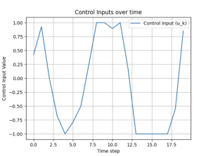
With the above parameters, we will solve the problem using MPC. Note that this example does not consider noises.

With the above formulation, we need to use a Kalman filter to estimate the state $\hat{x}(k)$ by observing the values of the measurements $y(k)$ .

The above equation can be easily formulated through the following MPC formulation:

$J = \sum_{i=0}^{N-1} \left( (\hat{x}(k+i) - x_{\text{ref}}(k+i))^T Q (\hat{x}(k+i) - x_{\text{ref}}(k+i)) \right) + \lambda \sum_{i=0}^{N-1} \left( u(k+i)^T R u(k+i) \right)$

The solution steps:

Initialization: start with the initial state $x(0)$ and the initial state estimate $\hat{x}(0)$
Kalman Filter Update: For each step, at each time step k, update the state estimate using the Kalman filter.
Prediction: For each step, predict future states using the state-space model and the updated state estimate.
Optimization: Solve the optimization problem to find the optimal control inputs.
Apply Control: Apply the first control input $u(k)$ to the system.
Update: Update the state $x(k+1)$ using the applied control input and repeat the process.

The solution code is shown below in part (3) Solutions

(2) Second Example: MPC with Kalman Filter Modeling

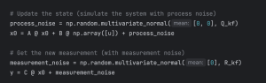
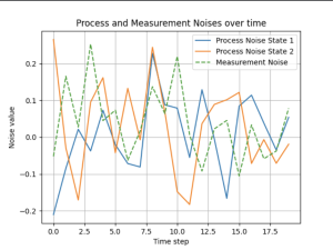
Given the same system with noises, the state space can presented as follows.

$A = \begin{bmatrix} 1 & 1 \\ 0 & 1 \end{bmatrix}, \quad B = \begin{bmatrix} 0 \\ 1 \end{bmatrix}, \quad C = \begin{bmatrix} 1 & 0 \end{bmatrix}$

We’ll define the process noise covariance $Q_kf$ and measurement noise covariance $R_kf$ as follows:

$Q_kf = \begin{bmatrix} 0.01 & 0 \\ 0 & 0.01 \end{bmatrix}, \quad R_kf = \begin{bmatrix} 0.01 \end{bmatrix}$

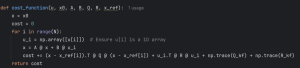
For the noisy system condition, once the process noises and measurement noises are in existence in the system, the cost function should consider it as well. The noises are the process noise covariance $Q_kf$ and measurement noise covariance $R_kf$ as follows:

$J = \sum_{i=0}^{N-1} \left( (x(k+i) - x_{\text{ref}}(k+i))^T Q (x(k+i) - x_{\text{ref}}(k+i)) + \text{tr}(Q_kf) \right) +... \\ ...+\lambda \sum_{i=0}^{N-1} \left( u(k+i)^T R u(k+i) + \text{tr}(R_kf) \right)$

where:

$x(k+i)$ is the predicted state at time step $k+i$
$x_{\text{ref}}(k+i)$ is the reference state at time step $k+i$
Q is the state weighting matrix
$u(k+i)$ is the control input at time step $k+i$
R is the control input weighting matrix
$\lambda$ is a weighting factor for the control effort
$\text{tr}(Q_{kf})$ is the trace of the process noise covariance matrix
$\text{tr}(R_{kf})$ is the trace of the measurement noise covariance matrix

The solution code is shown below in part (3) Solutions

(3) Solutions

Solution to first example: The code used to implement the MPC system without noises is shown in below. More specifically, the given state space without noises can be presented as follows.

Figure 14.3: The cost function of the noiseless MPC system.

Solution to second example: The noises are added to the system as shown below, both process noise and measurement noise. Note that, the process noise is added to the state equation since the process noise is more related to the physical conditions (states) of the system. However, the measurement noise is added to the output of the state space, since it is not state-related.

Figure 14.4: The cost function of the noisy MPC system.

Now that the system has noises, a Kalman filter is needed to filter the noises from the system. The Kalman filter predicates the states, updates the error covariance matrix, and calculates the Kalman gain.

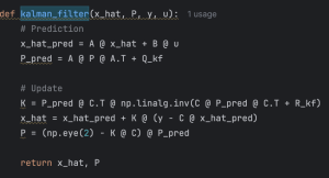
Figure 14.5: Kalman filter to filter the noises

The new cost function considering the noises is then used to replace the original cost function. Note that, the new cost function includes Q, the process noise covariance, and R, the measurement noise covariance.

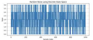
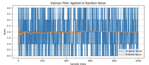
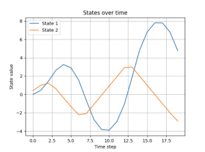
Figure 14.6: The cost function including the added process and measurement noises.

Following the process above, we can obtain the following state results. The two results correspond to the two different conditions where either no noises exist (Figure 14.7), or process and measurement noises are in existence (Figure 14.8).

Evidently, the results of the states and the input have both satisfied the constraints. Therefore, we can confidently say that the proposed MPC is effective in solving the state space while considering both process and measurement noises in the system.

Figure 14.7: The states of the noiseless system, X1 and X2.

Figure 14.8: The states of the noisy system, X1 and X2, and noises of the system.

Figure 14.9: The control input u of the system.

4) Class Engagement

Now you have learned the MPC theory, lets make summarization of the nature of the MPC controller. The key thing to implement MPC controller is to have optimal controller to solve the cost function a shown in below. Specifically, we use python package cvxpy to minimize the cost function.

$J = \sum_{i=0}^{N-1} \left( (x(k+i) - x_{\text{ref}}(k+i))^T Q (x(k+i) - x_{\text{ref}}(k+i)) \right) + \lambda \sum_{i=0}^{N-1} \left( u(k+i)^T R u(k+i) \right)$

Python Code:

cost += cvxpy.quad_form(x[:, t + 1], Q)
cost += cvxpy.quad_form(u[:, t], R)

The constrains needed to be satisfied is

$x(k+i+1|k) = A x(k+i|k) + B u(k+i)$

[x[:, t + 1] == A @ x[:, t] + B @ u[:, t]]

————— The Key Code of MPC in Python ————–

for t in range(T):
cost += cvxpy.quad_form(x[:, t + 1], Q)
cost += cvxpy.quad_form(u[:, t], R)
constr += [x[:, t + 1] == A @ x[:, t] + B @ u[:, t]]

Other Constains

$x_{\text{min}} \leq x(k+i|k) \leq x_{\text{max}}$

$u_{\text{min}} \leq u(k+i) \leq u_{\text{max}}$

where:

Python Code:

constr += [x[:, 0] == x0[:, 0]]

The below is to solve it with cvxpy.Minimize function

prob = cvxpy.Problem(cvxpy.Minimize(cost), constr)

We will use the same class engagment example as shown in the LQR chapter. For this problem, an inverted pendulum sits on a cart moving along the x-axis direction shown in Figure 14.10. The inverted pendulum can move along the X and Y direction. It means the inverted pendulum can swing back and forth shown.

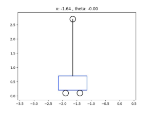
Figure 14.10 : Example of using Python to compute the LQR control gain K.

In order to control the inverted pendulum using LQR , we need to model the system. The followings show the process of the modeling

https://mtmailmtsu-my.sharepoint.com/:b:/g/personal/hbzhang_mtsu_edu/Ee-RhYhDtIRJqXFsQKpTBWoBq0Z9ZpVDy6PuTrdSbQzXYg?e=MPBRwJ

Through the derivation above, you can find the system state space as the following.

$\begin{bmatrix} \dot{x} \\ \ddot{x} \\ \dot{\theta} \\ \ddot{\theta} \end{bmatrix} = \begin{bmatrix} 0 & 1 & 0 & 0 \\ 0 & 0 & -\frac{gm}{M} & 0 \\ 0 & 0 & 0 & 1 \\ 0 & 0 & \frac{g(M+m)}{lM} & 0 \end{bmatrix} \begin{bmatrix} x \\ \dot{x} \\ \theta \\ \dot{\theta} \end{bmatrix} + \begin{bmatrix} 0 \\ \frac{1}{M} \\ 0 \\ \frac{1}{lM} \end{bmatrix} F$

Following running the code, results show that the use of LQR is able to stabilize the cart motion as shown in Figure 14.11. Specifically, when the cart is moving from one side to another, the inverted pendulum stays upright.

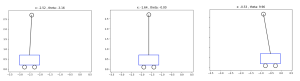
Figure 14.11: The results of running MPC python code showing that MPC is able to stablize the inverted pendulum on the moving cart.

License

Icon for the Creative Commons Attribution-NonCommercial-ShareAlike 4.0 International License

Robotics and Controls Engineering Copyright © by Hongbo Zhang; Elissa Ledoux; and Vishwas Bedekar is licensed under a Creative Commons Attribution-NonCommercial-ShareAlike 4.0 International License, except where otherwise noted.

1) Overview of Model Predictive Control

2) Using a Kalman Filter to Reduce Noise

(A) Prediction Step:

(B) Update Step:

3) Model Predictive Control (MPC) Modeling

(1) First Example: MPC with Kalman Filter Modeling

(2) Second Example: MPC with Kalman Filter Modeling

(3) Solutions

4) Class Engagement

License

Share This Book