Discrete State Space

Hongbo Zhang

12 Discrete State Space

Hongbo Zhang

1) Overview of Discrete State Space

Discrete state space is a powerful simplification of continuous state space. In some contexts, discrete state space is more useful for numerical computation, allowing us to more easily calculate the values of the states. As long as we can calculate the state values, we can do very powerful things with state space. In a controls context, we can control the system of interest.

2) Conversation of Continuous State Space to Discrete State Space

The conversion of continuous state space to discrete state space begins with the use of Laplace transforms to transform the state space from the time (“t”) domain to the frequency (“s”) domain using the Laplace transform $s = d/dt$ , as shown in Figure 1. The idea of using the Laplace transform is to solve for the state variables in the frequency domain. As shown in Figure 12.1, the state variable $X(s)$ is obtained through Laplace transform showing a relationship between $X(s)$ and $(sI-A)^{-1}$ . (As a reminder, $I$ is the identity matrix, which is multiplied by s in order to keep the equations in matrix form.)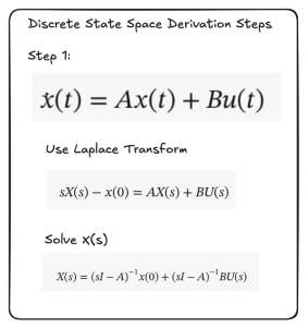

Figure 12.1: Step 1 of the conversion of continuous state space to discrete state space.

Following the Laplace transform, we can convert the equations back into the time domain using the inverse Laplace transform. After inverting the Laplace transform, we can obtain the inverse time domain equations of the state space, as shown in Figure 2. It is evident that $x(t)$ is a function of $e^{At}$ as shown in the bottom of Figure 12.2. However, only knowing $x(t)$ is insufficient; we are not yet in the discrete time domain. As such, we need to convert it to the discrete time domain.

Figure 12.2: Step 2 of the conversion of continuous state space to discrete state space.

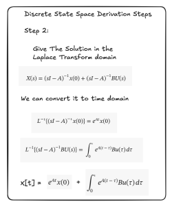
To convert to the discrete time domain, let us substitute the $X(t)$ with $X[k+1]$ . Note that once we convert $X(t)$ to $X[k+1]$ , we introduce the variables of $A_d$ and $B_d$ . While these two symbols are similar to $A$ and $B$ , the are actually not the same thing at all. $A_d$ and $B_d$ represent the state transition matrices. State transition matrix means that $A_d$ and $B_d$ can be used to transition the state $X(k)$ to its next time step $X[k+1]$ . Specifically, after integration, $B_d$ becomes $A^{-1} (A_d-I) B$ . By doing this, we have removed the integral here. Thus, it is easier to calculate $A_d$ and $B_d$ using this matrix operation, as shown in the bottom of Figure 12.3.

Figure 12.3: Step 3 of the conversion of continuous state space to discrete state space.

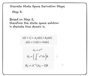
Now we are finally ready to convert the state space equations to the discrete time domain. Specifically, we are interested in solving the discrete time domain for $X(k)$ . To solve, we start from the results obtained from Step 3 as shown in Figure 12.3 above. There, we solved for $X[k+1]$ . As shown in Figure 12.4 below, $X[k+1]$ is both iterative and accumulative. As such, we can write easily the $X(k)$ equation shown in the middle of the figure. This equation is actually almost the final equation that we want to obtain: it is $X(k)$ ! However, this equation looks complicated. Why? It is because in the $X(k)$ equation in the middle of Figure 12.4, there is an $e^{AkT}$ term that makes the equation look very complicated and hard to calculate. So we must do one more step to simplify it a bit.

Figure 12.4: Step 4 of the conversion of continuous state space to discrete state space.

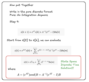
As shown in the bottom of the Figure 12.4, we have fully simplified the $X(k)$ equation. This simplification relies again on the state transition matrices:

$A = e ^{AT}$
$B = A^{-1}(e^{AT} - I) B$

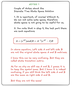
*Note that A and B on the left side of the equation are not the same as A and B on the right side, but for unknown reasons, the convention is to use the same symbols despite the fact that they represent different things. The A and B on the left side of 1. and 2. above correspond to $A_d$ and $B_d$ from Figure 12.3.*

$\newline$

The state transition matrix has successfully removed $e ^{AT}$ from the equation, as shown in Figure 12.4. It makes the calculation much more friendly. Why? It is because it has totally removed time from the equation. In this equation, we have only kept k as the changing value. This exactly matches our calculation goal of $X(k)$ , where the only changing value is $k$ . Therefore, we are done with the derivation.

$\newline$

The final equation of $X(k)$ is highlighted in the box with red outline shown in the bottom of Figure 12.4. In this $X(k)$ equation, we find that the $X(k)$ value only relies on k as the changing variable. Other matrices A and B are the state transition matrices, not the original state space A and B, which are the system matrix and the input matrix.

$\newline$

The beauty of this equation is that, as long as we know the original A and B matrices, which are the system matrix and input matrix, we only need to change the value of k to calculate all the $X(k)$ values. Therefore, we call it discrete state space. With the discrete state space values of $A, B,$ and k known, we can calculate all the discrete values of $X(k)$ . With these discrete values of $X(k)$ , it is possible for us to optimize the controller (aka optimize LQR).

3) Discussion of Discrete State Space Properties

The discrete solution of the state space is important. Without the discrete solution, we are not able to control the underlying system. It is also very interesting to note that the state transition matrix is particularly important, as noted in Figure 12.5. It shows the state space evolution process, thus providing insights for optimizing the control process.

Figure 12.5: First note for the conversion of continuous state space to discrete state space.

It is also useful to summarize the derivation process from continuous state space to discrete state space so that we can better understand the entire process. As shown in Figure 12.6, we have the original state space at the top; then following the derivation steps, we obtain the discrete state space. In the discrete state space, the values of $A_d$ and $B_d$ are presented. These are followed by the actual solution of $X[k]$ . For the equation of $X[k]$ , we have obtained the following coefficients $A$ and $B$ . These two coefficients are sufficient for us to calculate the discrete values of X[k] shown in Figure 12.6.

$A = e ^{AT}$
$B = A^{-1}(e^{AT} - I) B$

Figure 12.6: Second note for the conversion of continuous state space to discrete state space.

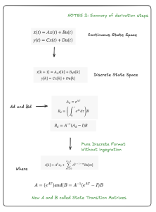
We can further simplify the derivation process of continuous state space to discrete state space using only two equations, as shown in Figure 12.7. The top of Figure 12.7 shows the discrete state space $x[k+1]$ and $x[k]$ . For this equation, $A$ and $B$ are still the system matrix and input matrix. The solution of the discrete state space is also illustrated in the bottom section of Figure 12.7. In the solution of $x[k]$ , however, the symbols of $A$ and $B$ are not the system and input matrices anymore; instead, they are the state transition matrices used to determine the values of the state space.

Figure 12.7: Third note for the conversion of continuous state space to discrete state space.

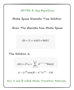
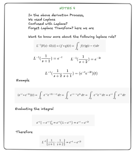
In the above derivation, it is possible that you may have felt confused about the derivation process of the Laplace transform, especially when it is used to calculate the Laplace transform of two functions multiplied together, as shown in Figure 12.8 below. This figure provides a review of the Laplace transform multiplication rule. This rule is critical when performing step 2 of the derivation for transforming the continuous state space to discrete state space (as in Figure 12.2 earlier).

Figure 12.8: Fourth note for the conversion of continuous state space to discrete state space.

4) Examples of Discrete State Space Computation

Hopefully, through the above steps, you now have a good understanding of the conversion of continuous state space to discrete state space. Now, it is time for us to illustrate the discrete state space calculation with some examples. Through these examples, you will understand how to actually use the discrete state space to do some meaningful tasks.

$\newline$

Figure 12.9 shows a simple example, where the coefficients A=0.9 and B=0.1. In this example, one can see that the calculation of the value of $x[k]$ is iterative. It means that the $x[k]$ value is dependent on the $x[k-1]$ value. As such, the $x[k]$ value is actually a summation of all values of the previous states.

$\newline$

From a control perspective, this is actually very interesting. It means that we need some control mechanisms to ensure that these accumulation effects will not make our control system diverge (go out of control). For PID control, we use an integral gain to accomplish this objective. For the first example, when A=0.9 and B=0.1, we can see that this will yield a constant value of $x[k]$ . It means that the value of $x[k]$ is just a constant number that will never change.

Figure 12.9: The first example of the discrete state space calculation.

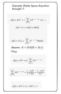
The second example also shows a simple example, where the coefficients A=0.7 and B=-9, shown in Figure 12.10. Apparently, with A=0.7 and B=-9, the values of $x[k]$ keep increasing. Therefore, this means that the underlying state space is unstable. In order to make the underlying system stable, we have to change the values of A and B. The use of feedback actually will be able to change A and B, therefore make the system stable.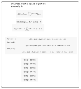

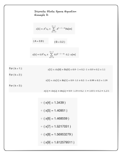
Figure 12.10: The second example of the discrete state space calculation.

Figure 12.11 shows another simple example, where the coefficients A=0.9 and B=0.2. Apparently, with A=0.9 and B=0.2, the values of $x[k]$ still keep increasing, but at a much smaller rate. This means that the underlying state space is still unstable, but it is much smoother and less wild in terms of the unstable dynamics. This helps us to gain some confidence that changing the $A$ and $B$ values is indeed useful to make the system more controllable and achieve a steady state.

Figure 12.11: Third Example of the discrete state space calculation.

License

Icon for the Creative Commons Attribution-NonCommercial-ShareAlike 4.0 International License

Robotics and Controls Engineering Copyright © by Hongbo Zhang; Elissa Ledoux; and Vishwas Bedekar is licensed under a Creative Commons Attribution-NonCommercial-ShareAlike 4.0 International License, except where otherwise noted.

1) Overview of Discrete State Space

2) Conversation of Continuous State Space to Discrete State Space

3) Discussion of Discrete State Space Properties

4) Examples of Discrete State Space Computation

License

Share This Book