
17 Ball Balancing Integral Control with Kalman Observer
Hongbo Zhang
Ball Balancing Project Background
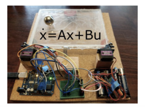
In this chapter, we will discuss an open source project available on Hackaday. The project is about controlling a ball balancing on a resistive touchscreen surface. The project link is listed below.
Ball Balancing Project Hackaday Link
The project is well done in a few aspects. First, the project is closely related to the state space applications in practical engineering control. Second, the author has released all the important project files to the control engineering community, which is very useful and beneficial to control engineering applications.
The project overall goal is to achieve the control of ball balancing on the resistive touch screen. The author has put a YouTube video link below to explain the project in detail.
Overall, we want to achieve the control of the system using the integral control technique. In contrast to the full state feedback controller, which suffers from the steady state error problem, integral control is able to reduce the steady state error of the system. As such, it becomes an effective approach for controlling the balance of the ball to enable it to stay at the center of the resistive touch screen.
Ball Balancing Project Control Theory
Luenberger Observer (Observer Taught in Class for Two Weeks and Lab 4)
The system involves the use of a Kalman observer to estimate the states and then remove the noise from the system. A Kalman observer is similar to a Luenberger observer. We learned about the Luenberger observer in the previous chapter of our class. Hopefully you understood it, but we will review the Luenberger observer again just in case.
It should be noted that in class, we did not call it a “Luenberger observer” much. Instead, we just called it an “observer” for convenience. Hopefully this new terminology has not confused you. A Luenberger observer is the default observer introduced in many textbooks. As such, people just tend to call it simply “observer” for convenience. The Luenberger is one of the simplest observers available to teach in control class.
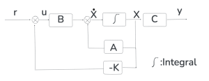
A full state feedback control diagram is shown below.
A Luenberger observer is shown below in the control diagram.
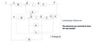
Figure 2 shows that we use full state feedback with an observer to implement the control using an observer. Note that there is an obvious benefit to use an observer on  rather than the original state X to achieve the control. First, we can save some sensors to not measure every single state. Instead, we just use the observer to estimate these states. Second, we can remove noise from the measured states.
The overall purpose of the Luenberger observer is to estimate the state so that we do not have to use many sensors to measure the states. The Luenberger observer shows that it is feasible to estimate the state of the plant through the use of the observer gain L matrix shown in Figure 2 above. With the observer gain L matrix, it becomes feasible to estimate .
Through the feedback process, with the feedback gain  , we do not use the original state
  anymore. Instead, we will use as the feedback.
The question is, why do we need to use the observer state rather than just simply using for the feedback as shown in the full state feedback control process? Note that contains the physical variables measured through the process, such as position, velocity, and acceleration for a mechanical system. The reason that we use rather than is because this way we do not suffer the problems associated with ; for example, the noise issue related to the . It also becomes feasible to reduce the number of sensors needed for the full state feedback process. Without the use of the observer in the control process, for the full state feedback controller to work, we would need to measure every single state to ensure the controller is able to work. Now, with the use of the observer, we can just use the observer to estimate the states, such as position, velocity, and acceleration. The benefit is that it will reduce the number of sensors needed to complete this wonderful control project.
The key equations associated with observer are:
The equation used to design observer gain L:
![\[ \dot{e} = (A - LC)e \]](https://mtsu.pressbooks.pub/app/uploads/quicklatex/quicklatex.com-aae984c545cd9126caaec5c562852d0e_l3.png "Rendered by QuickLaTeX.com")
The equation to show the estimated state :
![\[ \hat{x} = A\hat{x} + Bu + L(y - \hat{y}) \]](https://mtsu.pressbooks.pub/app/uploads/quicklatex/quicklatex.com-6f57a2d9516470dc544fc25f4a38f1d6_l3.png "Rendered by QuickLaTeX.com")
Full State Feedback Integral Control (Seen Lecture Notes, Last Group Quiz)
Very nice! It looks like you understand the observer better now. Now, it is time to diver deeper. As we hinted in the ball balancing project background section, we need to use integral control to remove the steady state error. We want the ball to stay at the center of the resistive touch screen. For this purpose, the use of only full state feedback is insufficient. Full state feedback control is not able to ensure zero steady state error. In order to do this, we need to use integral control. In order to use integral control, let us first review it. Note that the integral control here is similar to the integral control in the PID controller, but we return to this concept in state space based full state feedback control.
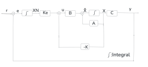
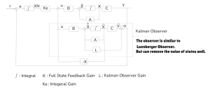
Integral control is very similar to the full state feedback control. However, it includes another outer feedback loop to feed back the output Y to the reference r. Note that the integral gain Ke is also involved here. With the integral gain, it becomes feasible to reduce the steady state error.
While integral control looks promising, it does not have an observer. This means that it still uses the raw states as the feedback. It therefore can not remove the noise of the states. To improve this situation, we need to use a Kalman observer to remove the noise. A Luenberger observer is not able to achieve this goal, so instead, we need to use a Kalman observer.
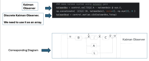
Kalman Observer Based Full State Integral Control
A Kalman observer is very similar to a Luenberger observer in principle, but it has the capability to remove noises from states. So often, we call it a Kalman filter instead of calling it a Kalman observer. Details of the mathematics of the Kalman observer can be referred to in the model predicative controller (MPC) chapter. In this case study, we will not focus on explaining the mathematics of the Kalman observer; rather, we will focus on how to implement it with python.
Ball Balancing Project Modeling and Implementation
This system can be described by the following state space:
(1) 
Where
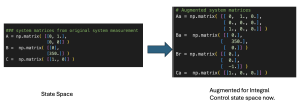
![\[ A = \begin{bmatrix} 0 & 1 \\ 0 & 0 \end{bmatrix}, \quad B = \begin{bmatrix} 0 \\ 350 \end{bmatrix}, \quad C = \begin{bmatrix} 1 \\ 0 \end{bmatrix} \]](https://mtsu.pressbooks.pub/app/uploads/quicklatex/quicklatex.com-8a2a715623b813dd7fe94d2581b148e9_l3.png "Rendered by QuickLaTeX.com")
![\[ A_a = \begin{bmatrix} 0 & 1 & 0 \\ 0 & 0 & 0 \\ 1 & 0 & 0 \end{bmatrix}, \quad B_a = \begin{bmatrix} 0 \\ 350 \\ 0 \end{bmatrix}, \quad B_r = \begin{bmatrix} 0 \\ 0 \\ -1 \end{bmatrix}, \quad C_a = \begin{bmatrix} 1 & 0 & 0 \end{bmatrix} \]](https://mtsu.pressbooks.pub/app/uploads/quicklatex/quicklatex.com-c14204ab10a87c126a6139117b149f65_l3.png "Rendered by QuickLaTeX.com")
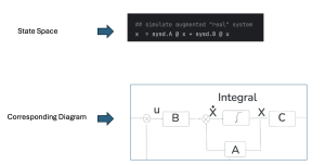
The state space in python can be represented as shown below.
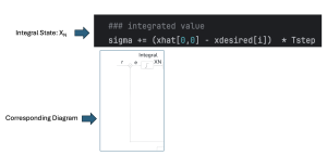
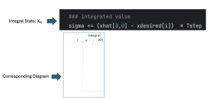
Specifically, we also explained the correspondence of the python code, the control theory, and the control diagram. This includes the integral state ( ), control input (u), state space, and Kalman observer.
The ball balancing integral control diagram is shown in the following. Now the question is how to use python to implement the control theory. The process is shown below step by step:
 ” using python and the related diagram.
Kalman Observer Based Full State Integral Control Results With Python and Arduino
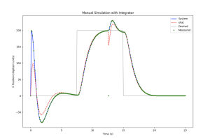
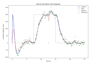
With the above control theory and python knowledge, it becomes possible that we can simulate the ball balancing system. In this simulation, we assume there is simulation and also assume there is noise condition, where noise can be equal to 0 and 10.
measuredX = x[0,0] + np.random.randn() * noise
After running the simulation, the output is shown in below. It is obvious that the use of Kalman observer is able to reduce the noises from the system.
You also can actually implement the Arduino code using Kalman Observer Based Full State Integral Control to control two servo motors. To make Arduino using the code to do this, we need to calculate the Kalman gain (L) and Integral gain (K) first using Python. Then we will use the the K and L computed with Python to do Arduino-based control. The Arduino code and results are shown below.
Arduino Code and Simulation Link
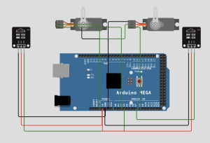
This exercise is very fun and informative. Please read the Arduino code carefully for how to use the Kalman gain (L) and Integral gain (K) to implement real-time Arduino-based ball balancing control precisely, using the Kalman Observer Based Full State Integral Control technique.
